The easiest way to plot ETG-4000 data in R is by using plot_ETG4000() from fnirsr package. However, if you want to explore your data in more detail, then an interactive plot is more appropriate.
I used dygraphs package to create the chart below. In case of using many channels, the colours in the legend can get a bit mixed up like in my example. I haven’t figured out yet how to add a custom colour palette that could deal with multiple channels.
One way or another, this code snippet should be enough to start generating interactive charts. I haven’t added the interactive chart to the main plotting function (i.e. plot_ETG4000) but I might do it in future releases.
The code used to generate the chart is here:
PS: The dygraph generated correctly in the interactive window, when using R notebooks, and when knitting. When I Saved as Web Page from RStudio, I got a header error that I had to clean by removing a tag (<!DOCTYPE html>) from the generated html file.
I haven’t worked on fnirsr (my R package for analysing fNIRS data) for a while so I thought it’s time for some improvements. I read a great introduction to Travis CI and decided to make it work this time. After running R CMD check (and devtools::check()) several times to fix multiple bugs, I finally got to see that lovely green badge 🙂
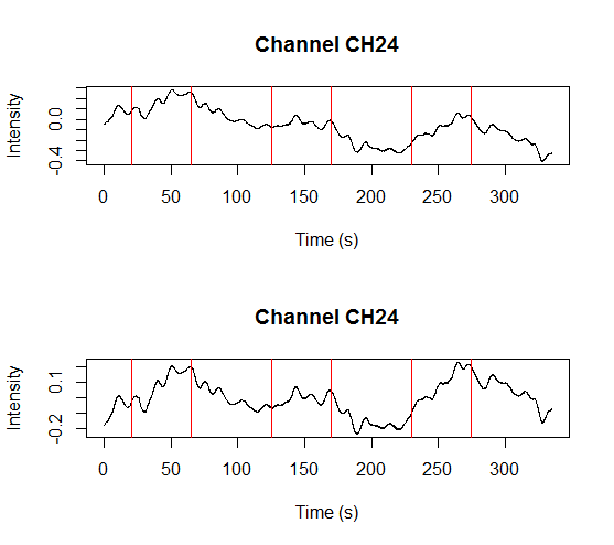
The package still needs more testing, but so far it does its job. On top of that, I finally added a function that removes a linear trend from an fNIRS signal:
For more details and the latest updates see the project’s GitHub page.
CRAN, here I come!
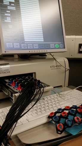
In the process of designing my latest experiment in PsychoPy I realised that setting up the serial port connection is not the most obvious thing to do. I wrote this tutorial so that others (and future me) won’t have to waste time reinventing the wheel.
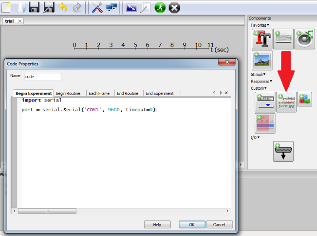
After creating an initial version of my experiment (looping over a wav file) I tried to figure out how to send a relevant trigger to my fNIRS. Luckily, the PsychoPy tutorial has a section about using a serial port, but after reading this I still wasn’t sure how to use the code with my script. After a quick brainstorm with the lab technician, we figured out that a simple script (see below) is indeed sending triggers to the fNIRS:
To better understand the arguments of the serial.Serial class please consult the pySerial documentation.
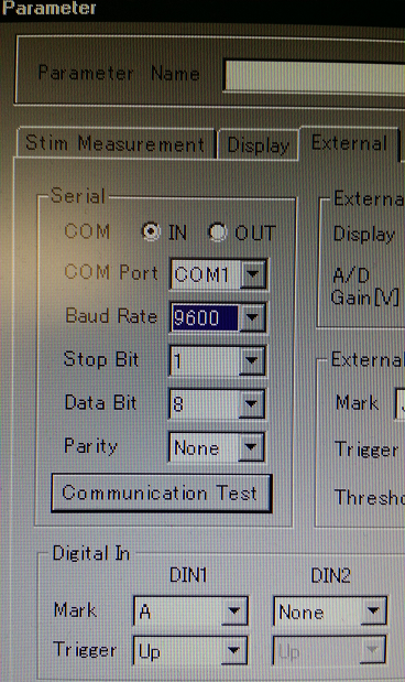
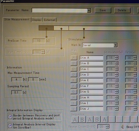
The argument (‘COM1’) is the name of the serial port used. The second argument is the Baud rate, it should be the same as the Baud rate used in the Parameter/External settings of the ETG-4000:
The last line of the script is sending the signal through the serial port. In this example, it is “A ” followed by Python’s string literal for a Carriage Return. That was one of the strings expected by ETG-4000, i.e. it was on the list previously set up in Parameter/Stim Measurement:
The easiest way for me to test whether I was sending correct signals was to use the Communication Test in the External tab (see the second screenshot). Once the test is started, you can run the Python script to test whether the serial signals are coming through.
If the triggers work as expected, the code sections for serial triggers can be embedded in the experiment. It can be done via GUI or code editor. That’s where to add code using GUI:
The next step is adding the triggers for the beginning, each stimulus/block, and the end of recording.
Here is an example of an experiment using serial port triggers to delimit blocks of stimuli and individual stimuli.
Due to the sampling rate, I had to add delay between the triggers delimiting the blocks, otherwise they would not be captured accurately. The triggers for block sections had to be send consecutively because the triggers cannot be interspersed (not sure if that’s because of my settings). For instance, AABBAA is fine, but ABABAB is not.
As I mentioned in my previous post, I am trying to get my head around analysing fNIRS data collected using Hitachi ETG-4000. The output of a recording session with ETG-4000 can be saved as a raw csv file (see the example). This file seems to be pretty straightforward to parse: the top section is a header, and raw data starts at line 41.
I created a set of basic R functions that can deal with the initial stages of the analysis and I wrapped them in an R-package. It is still a very early alpha (or rather pre-alpha), as the documentation is still sparse and no unit tests were made. I only have several raw csv files and they seemed to work fine with my functions but I’m not sure how robust they are.
Anyway, I think it will be useful to release it even in the early stage and work on the functions as time goes by.
The package can be found on GitHub and it can be installed with the following command:
devtools::install_github("erzk/fnirsr")
A vignette (Rmd) is here.
HTML vignette:
I couldn’t find any other R packages that would deal with these files so feel free to contact me if you work(ed) on something similar. Pull requests are encouraged.
Recently I started to learn how to use Hitachi ETG-4000 functional near-infrared spectroscopy (fNIRS) for my research. Very quickly I found out that, as usual in neuroscience, the main data analysis packages are written in MATLAB.
I couldn’t find any script to analyse fNIRS data in R so I decided to write it myself. Apparently there are some Python options, like MNE or NinPy so I will look into them in future.
ETG-4000 records data in a straightforward(ish) .csv files but the most popular MATLAB package for fNIRS data analysis (HOMER2) expects .nirs files.
There is a ready-made MATLAB script that transforms Hitachi data into the nirs format but it’s only available in MATLAB. I will skip the transformation step for now, and will work only with a .nirs file.
The file I used (Simple_Probe.nirs) comes from the HOMER2 package. It is freely available in the package, but I uploaded it here to make the analysis easier to reproduce.
My code is here:
This will produce separate time series plots for each channel with overlapping triggers, e.g.:
As a fan of both open data and ROH I was excited to find the article promising that the ROH’s data might be opened. However, this article was published in 2014 and the only open data about ROH that I could find was the Royal Opera House Collections Database. Its format is far from being user-friendly, i.e. there are no cleaned csv (or even xlsx) files, but luckily the structure of the entire website is fairly predictable. This meant I managed to write a basic scraper to extract the high level performance data. Unfortunately the database only contained data for the years 1946-2012.
The result is this interactive dashboard created in Tableau:
Highlights:
The number of performances in 1993 (159) started to approach the peak previously reached in 1951 (168 performances).
1998 and 1999 were years when ROH was being reconstructed.
The matinees started to become more popular in the noughties.
1968 was the last year of performances as the Covent Garden Opera Company.
Tosca was the most popular opera in the studied period with 187 performances.
La bohème was the most popular matinee.
The Kirov Opera was the third most popular company performing at the ROH with 33 appearances. After the name change to Mariinsky Theatre, there were additional four performances by this company.
I found a new dataset about UK broadband speeds and I started analysing it in R. However, after cleaning the data, I thought that creating a dashboard with Shiny would take me too much time so I moved to Tableau. I wanted to keep my analyses in one place so I embedded the dashboard into the output html document (see below).
Initially I thought that RMarkdown can’t generate embedded Tableau visualizations because the iframe in my report seemed blank after knitting the report. I had to open the generated in the browser to see the iframe filled with Tableau dashboard.
While working with UK geographical data I often have to extract geolocation information about the UK postcodes. A convenient way to do it in R is to use geocode function from the ggmap package. This function provides latitude and longitude information using Google Maps API. This is very useful for mapping data points but doesn’t provide information about UK-specific administrative division.
I got fed up of merging my list of postcodes with a long list of corresponding wards etc., so I looked for smarter ways of getting this info.
That’s how I came across postcodes.io which is free, open source, and based solely on open data. This service is an API to geolocate UK postcode and provide additional administrative information. Full documentation explains in details many available options. Among geographic information you can pull using postcodes.io are:
Postcode
Eastings
Northings
Strategic
County
District
Ward
Longitude
Latitude
Westminster Parliamentary Constituency
European Electoral Region (EER)
Primary Care Trust (PCT)
Parish (England)/ community (Wales)
LSOA
MSOA
CCG
NUTS
ONS/GSS Codes
I conduct most of my analyses in R so I developed wrapper functions around the API. Developmental version of the PostcodesioR package can be found on GitHub and documentation is here. It still doesn’t support all optional arguments but should do the job in most cases. A reference manual is here.
A mini-vignette (more to follow) showing how to run a lookup on a postcode, turn the result into a data frame, and then create an interactive map with leaflet:
The code above produces a data frame with key information
> glimpse(pc_df)

Observations: 1

Variables: 28

$ postcode                    EC1Y 8LX

$ quality                     1

$ eastings                    532544

$ northings                   182128

$ country                     England

$ nhs_ha                      London

$ longitude                   -0.09092237

$ latitude                    51.52252

$ parliamentary_constituency  Islington South and Finsbury

$ european_electoral_region   London

$ primary_care_trust          Islington

$ region                      London

$ lsoa                        Islington 023D

$ msoa                        Islington 023

$ incode                      8LX

$ outcode                     EC1Y

$ admin_district              Islington

$ parish                      Islington, unparished area

$ admin_county                NA

$ admin_ward                  Bunhill

$ ccg                         NHS Islington

$ nuts                        Haringey and Islington

$ admin_district              E09000019

$ admin_county                E99999999

$ admin_ward                  E05000367

$ parish                      E43000209

$ ccg                         E38000088

$ nuts                        UKI43
and an interactive map showing geocoded postcode as a blue dot:
One of my latest tasks at work was to analyse data related to Brexit referendum results and the UK housing market.
Luckily, all but rental data (acquired from Zoopla) was publicly available. Property prices and rental prices needed some wrangling as Land Registry doesn’t provide information about Local Authority districts, and that was the unit used by The Electoral Commission. LA districts are not a default geographic category in Tableau (version 9.3.5) but the official blog has recently featured a post demonstrating how to use non-standard mapping.
The final result was a map (below) and a press release. This is another housing market analysis that gained a lot of media coverage, among others by International Business Times, Business Insider, and Mortgage Introducer.
I wanted to dig deeper into the relationship between the voting pattern and the housing market information so I created the following bar charts:
Once the data is visualised in this way it becomes rather obvious that the areas where house prices and the capital gains (yearly average, in the last six years) were the highest, were also the ones that were the most likely to vote remain. The situation is much more difficult to interpret when the the results are sorted by the rental yields. In that case the voting pattern is not that clear anymore.
The scatter plots (and overlapping trend lines) make it easier to see the positive correlation between the percentage of people voting remain and the following variables: median house price (2016), median rental price (2016), and capital gains (yearly, across 2010-2016). This means that as the percentage of remain voters increases, so do the variables mentioned. This relationship did not hold for rental yields where it doesn’t seem to be any relationship between the two.
The Guardian and BBC conducted similar analyses comparing voting patterns to demographic variables.