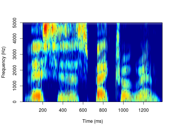
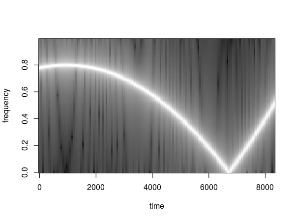
Creating a spectrogram is a basic step in every analysis of audio signals. Spectrograms visualise how frequencies change over a time period. Luckily, there is a selection of R packages that can help with this task. I will present a selection of packages that I like to use. This post is not an introduction to spectrograms. If you want to learn more about them then try other resources (e.g. lecture notes from UCL).
The examples shown below came mostly from the official documentation and were kept as simple as possible. The majority of functions allow further customisation of the plots.
phonTools
seewave
seewave and ggplot2
signal
soundgen
warbleR
hht
Creating a spectrogram from the scratch is not so difficult, as shown by Hansen Johnson in this blog post. Another solution was provided by Aaron Albin.
Praat is a workhorse of audio analysis. It is a standalone software, but there is also an R controller called PraatR, that allows calling Praat functions from R. It is not the easiest tool to use so I will just mention it here for reference.
I am pretty sure that there are more packages that allow creating spectrograms but I had to stop somewhere. Feel free to leave comments about other examples.
Homer2 needs a particular format of a .nirs file that cannot have consecutive triggers (also called Marks in Hitachi files).
hitachi2nirs Matlab script also removes the markers but I wanted to recreate the whole process and be sure that I’m doing it correctly. Answering Yes to the question Do you want to remove the marker at the end of each stimulus? y/n will run the following code:
To remove the triggers/markings in R follow the steps below.
and a plot showing raw data in one channel (quite noisy) with all the triggers.
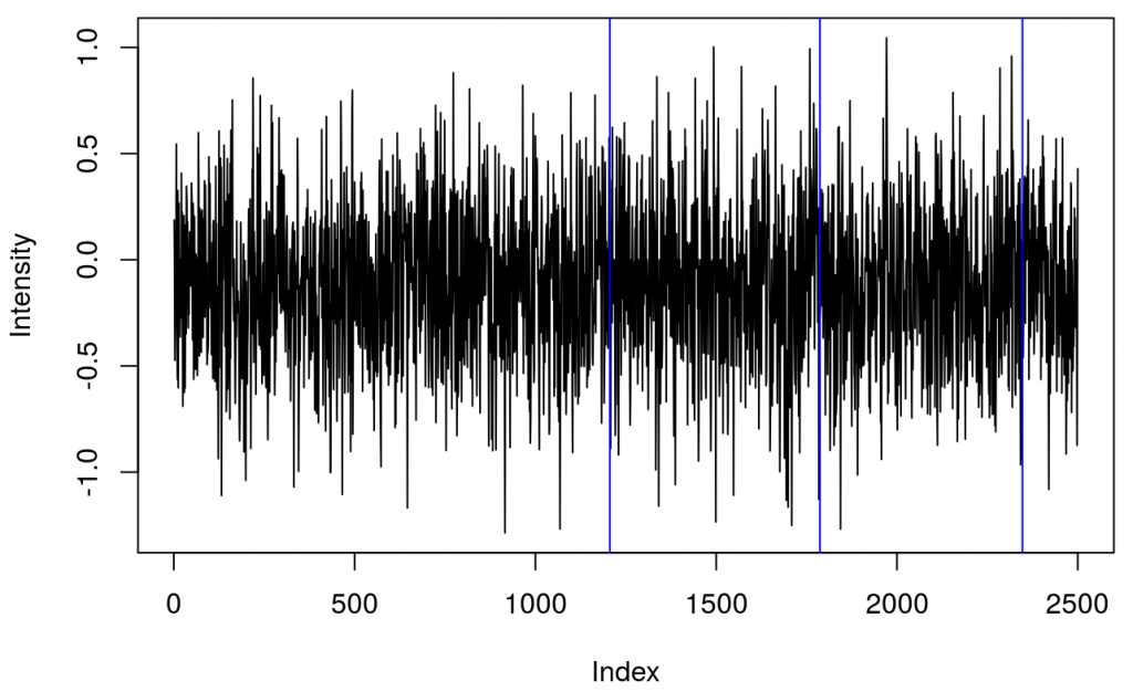
This shows several triggers (all plotted using red colour). I will only keep trigger ‘2’ to mark the beginning of a block. The first step is cleaning the data by removing all but trigger ‘2’.
Which results in fewer events
It turned out that there were two ‘2’ triggers next to each other. That’s because ETG-4000 does not allow odd triggers next to each other, e.g. 212 is invalid, but 22111122 is valid. I wrote a function (soon incorporated into fnirsr package) that deals with this problem.
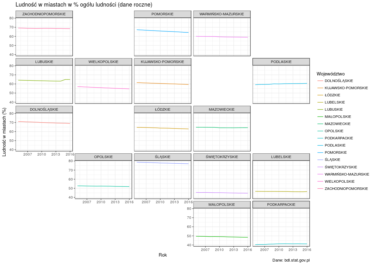
Niedawno odnalazłem ciekawy pakiet geofacet, który umożliwia rozmieszczenie wykresów zgodnie z ich pozycją na mapie. Główna funkcja facet_geo() zastępuje facet_wrap() z ggplot2. Polska mapa jeszcze nie jest dostępna w standardowym pakiecie geofacet, ale mam nadzieję, że już wkrótce tam się znajdzie, bo dodałem ją na GitHubie.
Stworzyłem siatkę z koordynatami poszczególnych województw. Wykresy z pakietem geofacet mogą wyglądać tak:
Rozmieszczenie województw nie jest idealne, ale pakiet geofacet umożliwia użycie własnych ustawień.
Dane pochodzą z Banku Danych Lokalnych (XLS - tablica przestawna)
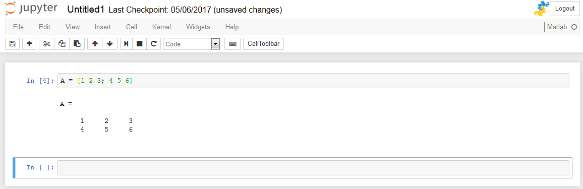
In my previous post I showed how to enable MATLAB in Jupyter notebooks on Windows. Now it’s time for GNU/Linux (Ubuntu).
My main issue with enabling new kernel was having initially installed two Anacondas and two Python versions (2.7 and 3.5). After a lot of frustration, I decided to remove both Anacondas and have a clear install of the latest Anaconda with Python 2.7 and 3.5. In this tutorial I assume that Jupyter and MATLAB are already installed on your system.
Using the right environment
Although the official MATLAB website states that Python-MATLAB engine works with Python 2.7, 3.4, 3.5 and 3.6, I struggled to install it using Python 3.5. If you try to install it with a 3.5 version, you will see the following error:
OSError: MATLAB Engine for Python supports Python version 2.7, 3.3 and 3.4, but your version of Python is 3.5
The error makes it obvious that you need an older version of Python. I decided to use 2.7. To do that, I created another environment with Python 2.7:
conda create -n py27 python=2.7 anaconda
The guidelines to managing Python environments are here.
The next step was checking what environments were available:
conda info --envs
And activating Python 2.7 (py27):
source activate py27
Install Python-MATLAB engine
To install the engine connecting both languages: go to your MATLAB folder, find the Python engine folder and install setup.py. This can be done in the following way:
Change your working directory to where your MATLAB lives: cd "MATLABROOT/extern/engines/python"
If you don’t know where your MATLAB is installed, use: locate matlab
Then install the engine (it will only work with MATLAB >=2014b):
That should do the job. Now open new Jupyter notebook:
jupyter notebook
To check whether you can find MATLAB among the available engines (top right corner):
Now check whether you can actually run the notebook. Initially, when I tried using Python 3.5, I could see MATLAB among the options but the kernels would die each time I tried running the MATLAB code. Moving to Python 2.7, as described in this tutorial, solved the problem.
If all works fine then the following notebook should generate correctly:
Even though I’m getting the MetaKernelApp error, the notebook continues to work correctly: [MetaKernelApp] ERROR | No such comm target registered: jupyter.widget.version
To leave the environment used to run the notebook, simply type:
source deactivate
Notes
Initially, I struggled a bit with making it all work so in the meantime I also tried installing Octave (a free equivalent of MATLAB). I’m not sure whether that installation helped me with running MATLAB within Jupyter.
While trying to install the engine I came across several errors. I guess that most of them were related to my OS configuration and all of them were solved by searching for the error message. One of the errors was:
Error:
[I 00:58:19.847 NotebookApp] KernelRestarter: restarting kernel (3/5)
/home/eub/anaconda3/bin/python: No module named matlab_kernel
This was due to installing the Python engine in the wrong environment (i.e. my default Python 3.5). It was solved by activating Python 2.7 and using it to install the Python-MATLAB engine.
I think that there is an alternative way to activate MATLAB in Jupyter, without Anaconda, would be to explicitly point the installer to the Python version that supports the Py-MATLAB engine.
In my case: sudo ~/anaconda/pkgs/python-2.7.13-0/bin/python2.7 setup.py install
You might also want install the engine in a non-default location. In that case, MATLAB has a solution to that problem and suggested installing Python in the home directory.
There is another Jupyter kernel (imatlab) engine that supposedly works with Python 3.5 and MATLAB R2016b+ but I haven’t tested it myself. As long as my current configuration works, I’m not planning to go through the hell of installing dependencies again.
After using R notebooks for a while I found it really unintuitive to use MATLAB in IDE. I read that it’s possible to use MATLAB with IPython but the instructions seemed a bit out of date. When I tried to follow them, I still could not run MATLAB with Jupyter (spin-off from IPython).
I wanted to conduct analyses of electroencephalographic (EEG) activity and the best plug-ins to do it (EEGLAB and ERPLAB) were written in MATLAB. I still wanted to use a programming notebook so I had to combine Jupyter and MATLAB.
I spent a bit of time setting it all up so I thought it might be worthwhile to share the process. Initially, I had three version of MATLAB (2011a, 2011b, and 2016b) and two versions of Python (2.7 and 3.3). This did not make my life easier of Windows 7.
Eventually, I only kept the installation of MATLAB 2016b to avoid problems with paths pointing to other versions. MATLAB’s Python engine works only with MATLAB 2014b or later so keeping the older versions could only cause problems.
Instructions
Install Anaconda (2.7)
Install MATLAB (>=2014b) - if you are a student then it’s very likely that your university bought a license. There is also a free MATLAB-like language called Octave, but I have not used with Jupyter. Apparently, it is possible to combine Octave with Jupyter. I’m going to focus exclusively on MATLAB in this post.
Install MATLAB’s Python engine - run as admin and follow the steps on the official site.
Once the engine was installed, I could move to installing metakernel, matlab_kernel, and pymatbridge. Go to Anaconda prompt (run as admin) and run pip install metakernel
In the Anaconda prompt run pip install matlab_kernel - this will use the development version of the MATLAB kernel.
Run pip install pymatbridge to install a connector between Python and MATLAB.
… voilà!
MATLAB should now be available in the list of available languages.
Once you choose it, you can start using it in a Jupyter notebook:
Issues
Obviously, thing were not always this smooth. Initially, I ran into problems with installing MATLAB’s Python engine. The official website suggested running the following code: cd "matlabroot\extern\engines\python"
python setup.py install
Which I did but it resulted in an error:
Luckily, the error message was clear so I had to point Python to run the 64-bit version. I double-checked my versions with: import platform
platform.architecture()
Which returned 64-bit as expected:
Using a command with full path to Python solved the problem:
Summary
I hope this will be useful. I have been messing with other issues which were pretty specific to my system so I did not include them here. Hopefully, these instructions will be enough to make MATLAB work with Jupyter.
PS: I have also explained how to use MATLAB with Jupyter on Ubuntu.
During the development of another R package I wasted a bit of time figuring out how to add code coverage to my package. I had the same problem last time so I decided to write up the procedure step-by-step.
Provided that you’ve already written an R package, the next step is to create tests. Luckily, devtools package makes setting up both testing and code coverage a breeze.
Let’s start with adding an infrastructure for tests with devtools: library(devtools)
use_testthat()
Then add a test file of your_function() to your tests folder: use_test("your_function")
Then add the scaffolding for the code coverage (codecov) use_coverage(pkg = ".", type = c("codecov"))
After running this code you will get a code that can be added to your README file to display a codecov badge. In my case it’s the following: [](https://codecov.io/github/erzk/PostcodesioR?branch=master)
This will create a codecov.yml file that needs to be edited by adding: comment: false
language: R
sudo: false
cache: packages
after_success:
- Rscript -e 'covr::codecov()'
Now log in to codecov.io using the GitHub account. Give codecov access to the project where you want to cover the code. This should create a screen where you can see a token which needs to be copied:
Once this is completed, go back to R and run the following commands to use covr:
The last line will connect your package to codecov. If the whole process worked, you should be able to see a percentage of coverage in your badge, like this:
Click on it to see which functions are not fully covered/need more test:
I hope this will be useful and will save a lot of frustrations.
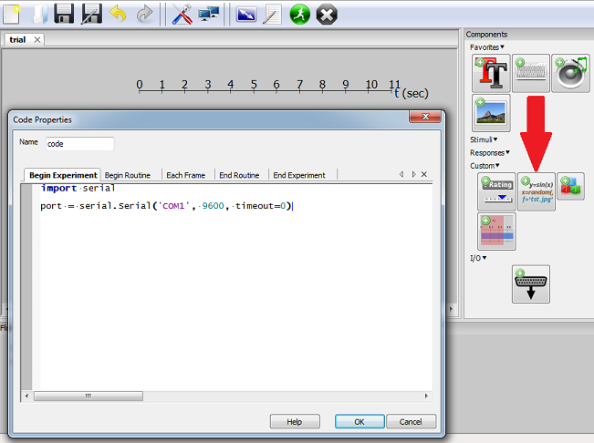
In the process of designing my latest experiment in PsychoPy I realised that setting up the serial port connection is not the most obvious thing to do. I wrote this tutorial so that others (and future me) won’t have to waste time reinventing the wheel.
After creating an initial version of my experiment (looping over a wav file) I tried to figure out how to send a relevant trigger to my fNIRS. Luckily, the PsychoPy tutorial has a section about using a serial port, but after reading this I still wasn’t sure how to use the code with my script. After a quick brainstorm with the lab technician, we figured out that a simple script (see below) is indeed sending triggers to the fNIRS:
To better understand the arguments of the serial.Serial class please consult the pySerial documentation.
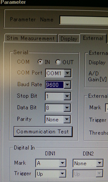
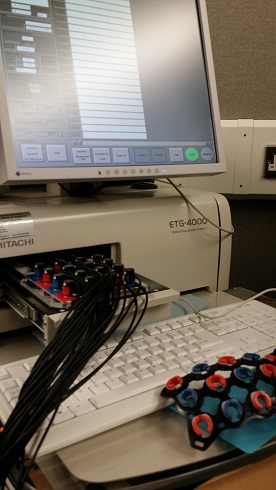
The argument (‘COM1’) is the name of the serial port used. The second argument is the Baud rate, it should be the same as the Baud rate used in the Parameter/External settings of the ETG-4000:
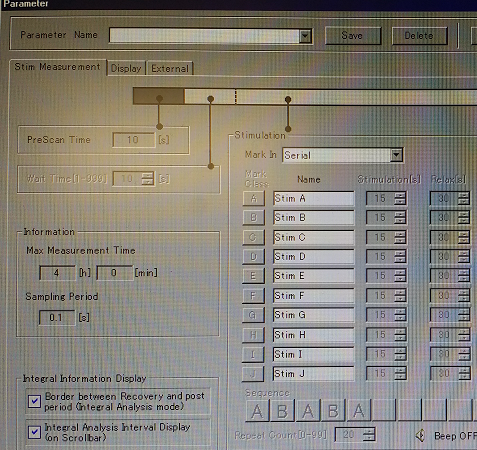
The last line of the script is sending the signal through the serial port. In this example, it is “A ” followed by Python’s string literal for a Carriage Return. That was one of the strings expected by ETG-4000, i.e. it was on the list previously set up in Parameter/Stim Measurement:
The easiest way for me to test whether I was sending correct signals was to use the Communication Test in the External tab (see the second screenshot). Once the test is started, you can run the Python script to test whether the serial signals are coming through.
If the triggers work as expected, the code sections for serial triggers can be embedded in the experiment. It can be done via GUI or code editor. That’s where to add code using GUI:
The next step is adding the triggers for the beginning, each stimulus/block, and the end of recording.
Here is an example of an experiment using serial port triggers to delimit blocks of stimuli and individual stimuli.
Due to the sampling rate, I had to add delay between the triggers delimiting the blocks, otherwise they would not be captured accurately. The triggers for block sections had to be send consecutively because the triggers cannot be interspersed (not sure if that’s because of my settings). For instance, AABBAA is fine, but ABABAB is not.
As I mentioned in my previous post, I am trying to get my head around analysing fNIRS data collected using Hitachi ETG-4000. The output of a recording session with ETG-4000 can be saved as a raw csv file (see the example). This file seems to be pretty straightforward to parse: the top section is a header, and raw data starts at line 41.
I created a set of basic R functions that can deal with the initial stages of the analysis and I wrapped them in an R-package. It is still a very early alpha (or rather pre-alpha), as the documentation is still sparse and no unit tests were made. I only have several raw csv files and they seemed to work fine with my functions but I’m not sure how robust they are.
Anyway, I think it will be useful to release it even in the early stage and work on the functions as time goes by.
The package can be found on GitHub and it can be installed with the following command:
devtools::install_github("erzk/fnirsr")
A vignette (Rmd) is here.
HTML vignette:
I couldn’t find any other R packages that would deal with these files so feel free to contact me if you work(ed) on something similar. Pull requests are encouraged.
Recently I started to learn how to use Hitachi ETG-4000 functional near-infrared spectroscopy (fNIRS) for my research. Very quickly I found out that, as usual in neuroscience, the main data analysis packages are written in MATLAB.
I couldn’t find any script to analyse fNIRS data in R so I decided to write it myself. Apparently there are some Python options, like MNE or NinPy so I will look into them in future.
ETG-4000 records data in a straightforward(ish) .csv files but the most popular MATLAB package for fNIRS data analysis (HOMER2) expects .nirs files.
There is a ready-made MATLAB script that transforms Hitachi data into the nirs format but it’s only available in MATLAB. I will skip the transformation step for now, and will work only with a .nirs file.
The file I used (Simple_Probe.nirs) comes from the HOMER2 package. It is freely available in the package, but I uploaded it here to make the analysis easier to reproduce.
My code is here:
This will produce separate time series plots for each channel with overlapping triggers, e.g.: