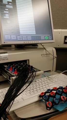
As I mentioned in my previous post, I am trying to get my head around analysing fNIRS data collected using Hitachi ETG-4000. The output of a recording session with ETG-4000 can be saved as a raw csv file (see the example). This file seems to be pretty straightforward to parse: the top section is a header, and raw data starts at line 41.
I created a set of basic R functions that can deal with the initial stages of the analysis and I wrapped them in an R-package. It is still a very early alpha (or rather pre-alpha), as the documentation is still sparse and no unit tests were made. I only have several raw csv files and they seemed to work fine with my functions but I’m not sure how robust they are.
Anyway, I think it will be useful to release it even in the early stage and work on the functions as time goes by.
The package can be found on GitHub and it can be installed with the following command:
devtools::install_github("erzk/fnirsr")
A vignette (Rmd) is here.
HTML vignette:
I couldn’t find any other R packages that would deal with these files so feel free to contact me if you work(ed) on something similar. Pull requests are encouraged.
Recently I started to learn how to use Hitachi ETG-4000 functional near-infrared spectroscopy (fNIRS) for my research. Very quickly I found out that, as usual in neuroscience, the main data analysis packages are written in MATLAB.
I couldn’t find any script to analyse fNIRS data in R so I decided to write it myself. Apparently there are some Python options, like MNE or NinPy so I will look into them in future.
ETG-4000 records data in a straightforward(ish) .csv files but the most popular MATLAB package for fNIRS data analysis (HOMER2) expects .nirs files.
There is a ready-made MATLAB script that transforms Hitachi data into the nirs format but it’s only available in MATLAB. I will skip the transformation step for now, and will work only with a .nirs file.
The file I used (Simple_Probe.nirs) comes from the HOMER2 package. It is freely available in the package, but I uploaded it here to make the analysis easier to reproduce.
My code is here:
This will produce separate time series plots for each channel with overlapping triggers, e.g.:
While working with UK geographical data I often have to extract geolocation information about the UK postcodes. A convenient way to do it in R is to use geocode function from the ggmap package. This function provides latitude and longitude information using Google Maps API. This is very useful for mapping data points but doesn’t provide information about UK-specific administrative division.
I got fed up of merging my list of postcodes with a long list of corresponding wards etc., so I looked for smarter ways of getting this info.
That’s how I came across postcodes.io which is free, open source, and based solely on open data. This service is an API to geolocate UK postcode and provide additional administrative information. Full documentation explains in details many available options. Among geographic information you can pull using postcodes.io are:
Postcode
Eastings
Northings
Strategic
County
District
Ward
Longitude
Latitude
Westminster Parliamentary Constituency
European Electoral Region (EER)
Primary Care Trust (PCT)
Parish (England)/ community (Wales)
LSOA
MSOA
CCG
NUTS
ONS/GSS Codes
I conduct most of my analyses in R so I developed wrapper functions around the API. Developmental version of the PostcodesioR package can be found on GitHub and documentation is here. It still doesn’t support all optional arguments but should do the job in most cases. A reference manual is here.
A mini-vignette (more to follow) showing how to run a lookup on a postcode, turn the result into a data frame, and then create an interactive map with leaflet:
The code above produces a data frame with key information
> glimpse(pc_df)

Observations: 1

Variables: 28

$ postcode                    EC1Y 8LX

$ quality                     1

$ eastings                    532544

$ northings                   182128

$ country                     England

$ nhs_ha                      London

$ longitude                   -0.09092237

$ latitude                    51.52252

$ parliamentary_constituency  Islington South and Finsbury

$ european_electoral_region   London

$ primary_care_trust          Islington

$ region                      London

$ lsoa                        Islington 023D

$ msoa                        Islington 023

$ incode                      8LX

$ outcode                     EC1Y

$ admin_district              Islington

$ parish                      Islington, unparished area

$ admin_county                NA

$ admin_ward                  Bunhill

$ ccg                         NHS Islington

$ nuts                        Haringey and Islington

$ admin_district              E09000019

$ admin_county                E99999999

$ admin_ward                  E05000367

$ parish                      E43000209

$ ccg                         E38000088

$ nuts                        UKI43
and an interactive map showing geocoded postcode as a blue dot:
Kaggle released another interesting data set. This time it’s a loan book of a P2P lender - Lending Club.
I had a stab at analysing it and here are some teaser charts that were created, but more can be found here.
R has a number of libraries that can be used for plotting. They can be combined with open GIS data to create custom maps.
In this post I’ll demonstrate how to create several maps.
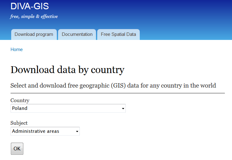
First step is getting shapefiles that will be used to create maps. One of the sources could be this site, but any source with open .shp files will do.
Here I’ll focus on country level (administrative) data for Poland.
If you follow the link to diva-gis you should see the following screen:
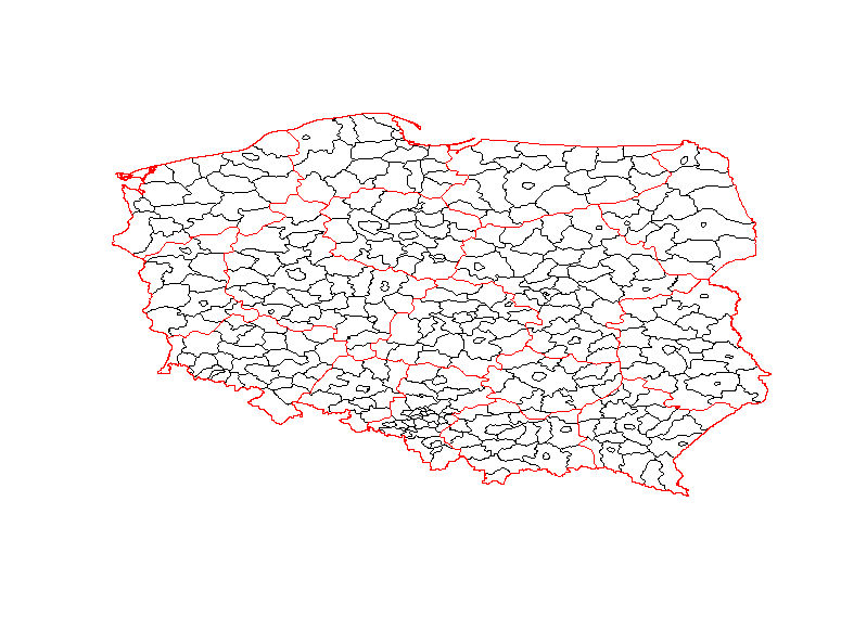
I’ll plot powiats and voivodeships which are first- and second-level administrative subdivisions in Poland.
After downloading and unzipping POL_adm.zip into your working directory in R you will be able to use the scripts underneath to recreate the maps.
The simplest map is using only the shapefiles without any extra background.
Clearly, it’s not the most attractive map, but it’s still informative.
It was generated with the following code:
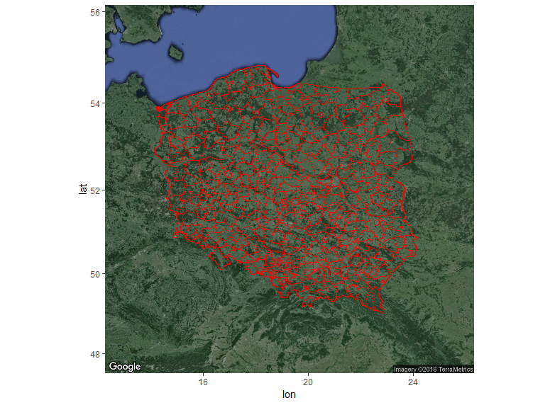
Nicer maps can be generated with ggmap package. This package allows adding a shapefile overlay onto Google Maps or OSM. In this example I used get_googlemap function, but if you want other background then you should use get_map with appropriate arguments.
Code used to generate the map above:
And last, but not least is my favourite interactive map created with leaflet.
Snippet:
> sessionInfo()

R version 3.2.4 Revised (2024-03-16 r70336)

Platform: x86_64-w64-mingw32/x64 (64-bit)

Running under: Windows 7 x64 (build 7601) Service Pack 1
Praat is a great tool for analysing speech data but lately I came across a frustrating problem. While trying to open a txt file (vector of numbers) in Praat I would get the following error message: File not recognized. File not finished.
After consulting my fellow PhD students I discovered that what I was missing was a header enabling Praat to read txt files.
The simplest way to fix this error is to add the following header to a text file using your favourite text editor:
However, if you want to automate the process then scripting can save you a lot of time. That’s why I created a function (txt2praat.R) appending this header to the original text file and saving the output to a new text file.
You can use the function in the following way: txtfile <- file.choose() txt2praat(txtfile, testfile-modified)
These commands should create a txt file (testfile - modified) appended with the short header. New file can be then opened in Praat without the error message.
Tableau Desktop 9.1 is out and Web Data Connectors are available as a new data source in this version. Luckily Tableau released several working connectors to popular web data sources and Google Sheets is one of them. Today I tried to connect to Google Sheets but I couldn’t find a step-by-step description of setting it up and the official thread lacked details about configuring WDC. It took me a while to figure out how to start using Web Data Connectors so I decided to write this tutorial which hopefully will help others to start using Web Connectors. This tutorial describes how to use Tableau web connectors hosted locally.
Before starting to use Web Data Connectors you need to activate Internet Information Services (IIS) Manager (more info available in this Stackoverflow thread).
This can be done on Windows 10 by pressing Windows key and typing Windows Features.
Then go to Turn Windows Features On or Off, and tick the box next to Internet Information Services.
Now you should be able to see IIS in Control Panel > Administrative Tools.
Open IIS Manager to check the values in Binding and Path columns. Binding should be set to *:8888 (http). Path points to a folder where the Tableau Connector files should be stored.
If Binding is set to a different value than 8888 (mine was set to 80 by default) then go to Actions on click on Bindings.
Then change the Port number to 8888 and click OK.
Now your IIS Manager configuration should look like this
Check the value of the Path column. It’s set to %SystemDrive%\inetpub\wwwroot by default which in most cases means C:\inetpub\wwwroot
In order to start using Google Sheets as a data source you need to start with downloading the Web Data Connector SDK.
Unzip the zip file and go to the Examples folder.
Copy all files from the Examples folder to the Path specified in IIS. In my case it was C:\inetpub\wwwroot
Now you should be ready to start using Web Data Connectors. Go to Connect > To a server > Web Data Connector
A pop-up window like the one below should appear
If you copied the example files provided by Tableau to your IIS path then type the following into the address bar of the WDC pop-up window: http://localhost:8888/GoogleSheetsConnector.html
You should see the following window
All you need to do now is to provide a link to a Google Sheet you want to use. You might also need to log into your Google Account if a Sheet provided is private.
Now you can start using Google Sheets as a data source. Hooray!
If you need to use other connectors then just change the path in the Address bar of the pop-up window.
Quandl is a great provider of various types of data that can be easily integrated with R. I wanted to play with the available data and see what kind of insights can be gathered using R.
I wrote a short script that collects British Pound Sterling (GBP) to Polish Złoty (PLN) historic exchange rates from 1996 till today (4th September 2015).
First thing I did was loading the libraries that will be used:
Then I downloaded the exchange rates data from Quandl. Data can be downloaded in several popular formats (i.e. ts, xts, or zoo), each appropriate for different packages.
Once I collected my data, I started cleaning the data frame that was downloaded from Quandl.
The column names designating High and Low Rates had whitespaces in them, and that could cause all sorts of problems in R. I removed ‘High_est’ and ‘Low_est’ from the xts data to make plotting with dygraphs easier. Thanks for lubridate package I easily extracted years, months, and days from the Date field. I also added a ‘Volatility’ column that showed the difference between the High and Low rates.
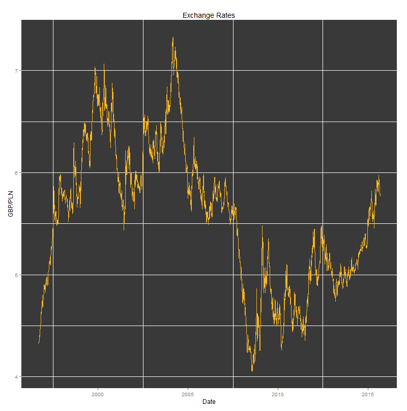
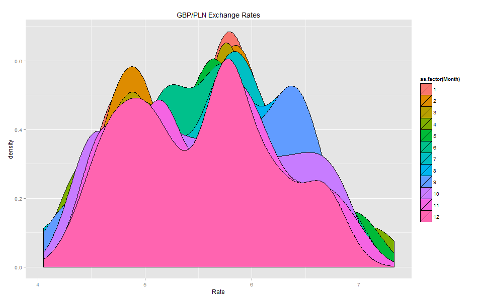
Now I had all my data cleaned so I could start plotting. I started by shamelessly copying the code for the Reuters-like plot that was included in Quandl’s cheat sheet. GBP/PLN Historic Exchange Rates
All plots were created using the following code:
The results can be seen underneath.
Density plots:
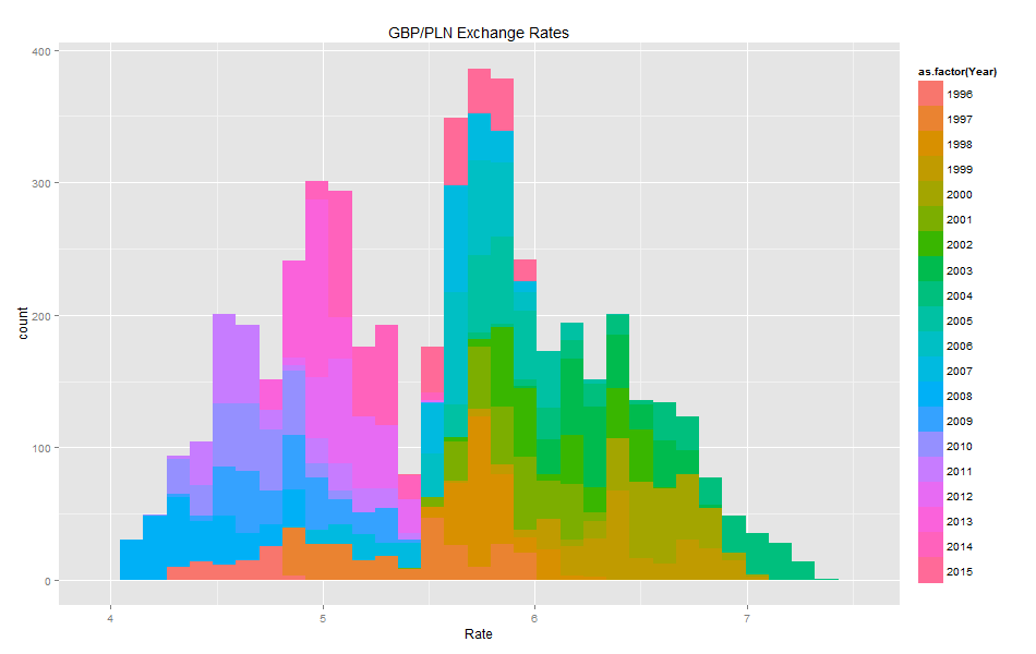
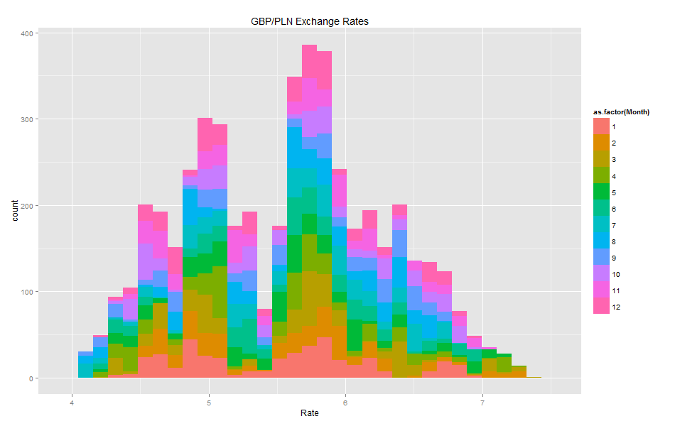
Histograms:
Volatility histogram shows clearly that there are many fields with missing values. GBP/PLN Volatility
Comparing the blank fields with those containing non-zero values showed that the number of blank vs. non-blank is almost the same. This means that Volatility should not be used as it has a high number of missing values.
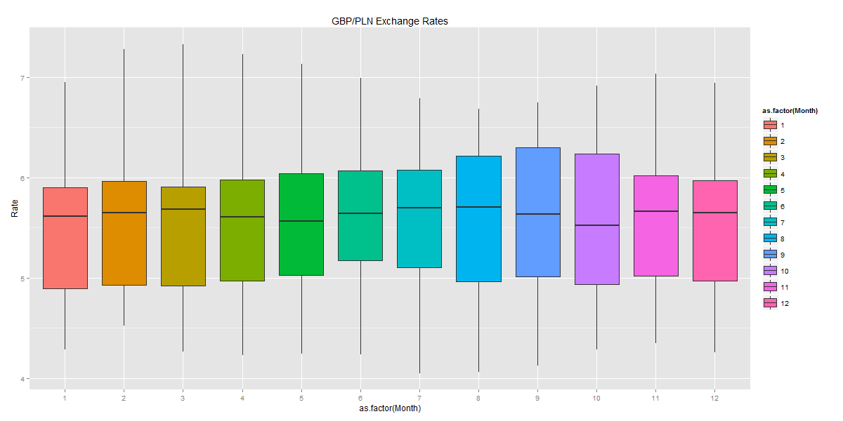
The box plots show how the GBP/PLN exchange rates fluctuate across different years and months. They also include the mean values and the variation in the exchange rates.
Last, but not least was the interactive plot created with dygraph package. That’s definitely my favourite as it allows fine-grained analysis of the underlying information (including date range selection).
I added the event lines that seemed to be relevant to the the observed maximum and minimum values of the GBP/PLN exchange rates. Around the time when Poland joined the EU, the GBP/PLN exchange rate peaked at 7.3 PLN. Four years later, just before Lehman Brothers went bankrupt, Pound Sterling was valued as low as 4.07 PLN.
The interactive plot was created using the following code:
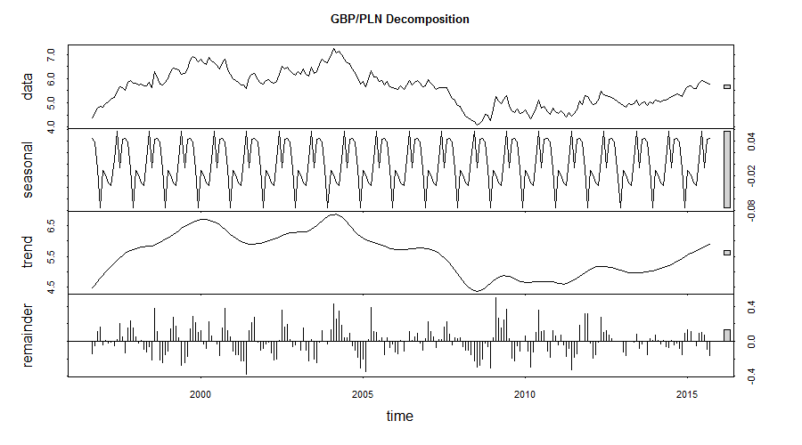
I thought that I had enough simple plots and now was the right time for more complicated analyses. I started with the Seasonal Decomposition of Time Series by Loess using the stl function.
GBP/PLN Seasonal Decomposition of the Historic Exchange Rates
Seasonal, trend and irregular components were extracted from the underlying data. The main trend is showing the appreciation of GBP against PLN but the seasonal component might be (?) indicating approaching correction of that trend.
I wanted to finish the analysis with applying the Anomaly Detection package, that was released by Twitter’s engineering team, to my data collected from Quandl. My plan was to see whether there were any anomalous changes of the exchange rate during the recorded period.
Running this code resulted in obtaining one anomalous value, i.e. 7.328 PLN, which was the maximum value observed in the collected time series.
I hope that you enjoyed this walkthrough. In future posts I want to descibe more ways to analyse time series.
I needed to extract mean pitch values from audio recordings of human speech, but I wanted to automate it and easily recreate my analyses so I wrote a couple of scripts that can do it much faster.
Here is a recipe for extracting pitch from voice recordings.
Cleaning audio files
My audio files were stereo recordings of a participant saying /a/ while hearing (near) real-time pitch shifts in their own productions. The left channel contains the shifted pitch (heard by participants) and the right channel contains the original speech productions.
The first step is to examine the audio recordings for any non-speech sounds. I used Audacity for that. Any grunts or sights can mess up the outcome of scripts used in the analysis. Irrelevant parts of the audio track can be silenced (CTRL+L in Audacity). Once the audio track is cleaned, I split the channels and save them in separate wav files.
Acoustic signal used in the analysis. Highlighted part is showing noise that should be removed.
Splitting continuous recordings using SFS
My pitch-extracting scripts expects each utterance to be saved in a separate wav file so I need to split the continuous recordings. It could be done manually but for longer recordings it’s cumbersome. Speech Filing System (SFS) has an option that allows splitting the continuous files on silence.
Specify the values of npoint. More information can be found here. You don’t need to know the exact number of utterances, but a close approximation should work.
Visualise the results of automatic annotation:
Check if the annotations are correct. If not, then tweak the npoint settings to get the effect you need.
3. Chop the files on annotations
Tools > Speech > Export > Chop signal into annotated regions
This will save the files in the sfs format, but PraatR can’t work with these files. They need to be transformed into wav.
4. Convert sfs into wav files
Load the files you want to convert, highlight them, and go to:
File > Export > Speech
Automatic:
If you don’t want to spend hours doing what I’ve just described then a simpler solution is using a program that runs all the commands described above.
Use the batch script that follows the steps described above (plus some extras).
Extracting mean pitch using PraatR
Pitch could be extracted manually in Praat by going to
View & Edit > Pitch > Get pitch
but doing this for many files would take a lot of time and would be error-prone.
Luckily, there is a connection between Praat and R (PraatR) which can speed up this task.
I extracted mean pitch and duration of files. The latter can be used to reject any non-speech files. Here’s the script:


